Energy Equation in Flow Systems

When energy crosses the boundary of a system, the energy in the system changes by an equal amount. Thus a decrease in the energy of a system equals the increase in energy of the surroundings and vice versa.

Energy can cross a system boundary in the form of heat transfer (to or from the system), in the form of work (done by or on the system), or by mass entering or leaving. A process during which no heat is transferred to or from a system is known as an adiabatic process. The law of conservation of energy states that for a system of particles

E₂ – E₁ = Q͂ - Wʹ

Or

dE = d Q͂ - dWʹ

Where:

• E2 – E1: is the change in energy experienced by the system
• Q͂: is the heat added to the system
• Wʹ: is work done by the system

The total energy is a property of the system and includes internal (U), kinetic (KE), and potential energies (PE):

E = U + KE + PE

If we express this on a per-unit-mass basis, we obtain:

Heat and work are not properties of the system, but they represent energy transfers moving across the system boundaries in specific forms.

Remember the general conservation expression:

If we substitute, N = E and n = e, we obtain:

Equation 1 is generally known as the first law of thermodynamics and is a statement of the conservation of energy.

The Wʹ term consists of all forms of work crossing the boundary. This includes shaft work, electric and magnetic work, viscous shear work, and flow work. The last of these forms represents work done by the fluid system in pushing mass into or out of the control volume. Thus:

where dW_f /dt is flow work per unit time.

To develop an expression for dW_f/dt, we can consider an element of mass dm leaving a control volume through an area dA, as shown below:

The fluid in the control volume must work against the external pressure p to move dm out. Since work = force x distance, we have:

Similarly, for an element of mass entering, work is being done on the system. Therefore, we get:

Combining the previous two equations, we can obtain the flow work as:

If we substitute Equations 3 and 2 into Equation 1 we get:

Combining the integral terms results in:

Enthalpy is a property defined as h = u + p/ρ; the conservation of energy equation now becomes:

For a steady, one-dimensional flow, the energy equation becomes:

For many incompressible flows, Q͂ is usually assumed to be zero, and changes in internal energy are frequently negligible. Thus equation 5 can be simplified into:

For compressible flows, however, the change in internal energy is significant and cannot be neglected. 

Momentum Equation

From the previous chapter, we saw that the continuity equation is a conservation of mass equation with which mass transfers across boundaries and mass storage within control volumes can be accounted for.

Now we can derive a conservation of linear and angular momentum equations using the same technique.

Linear Momentum Equation

Using the general conservation equation below:

(S = System, CV = Control volume, CS = Control surface)

Let N be momentum mV, and n, which is N per unit mass, becomes V. Thus, the general conservation equation becomes:

From Newton’s law for the system, we have:

Combining these equations with Equation 1, we get a conservation of linear momentum equation for the three principal directions:

Two velocity terms appear in the integrals of the last terms on the right-hand sides of equations 2a, 2b and 2c. One of the velocities refers to a principal flow direction; for example, V_x. The other velocity, V_n, is normal to the control surface where mass crosses the boundary. These two velocities are not always equal. Because force and velocity have magnitude and direction, they are vectors.

Thus, Equation 2 can be written in vector form as:

This equation is a conservation of linear momentum equation.

As required by Newton’s law, the term ΣF represents all forces applied externally to the control volume. These include forces due to gravity, electric and magnetic fields, surface tension effects, pressure forces, and viscous forces (friction).

The first term on the right-hand side of equation 3 represents the rate of storage of linear momentum in the control volume. The last term is a net rate out (out minus in) of linear momentum from the control volume. For steady one-dimensional flow, Equation 3 becomes, for any direction i,

For one fluid stream entering and one leaving the control volume, we have the following for one-dimensional flow:

The momentum equation can be used to set up a general equation for frictional effects existing within a pipe, for a certain type of phenomenon in open channel flow, and for other kinds of applications-oriented problems.

Angular Momentum Equation

For some fluid mechanics problems, it is essential to be able to evaluate moments exerted by moving fluid volumes especially for rotating machinery like turbines and pumps. The equation applicable to these instances is known as angular momentum equation and is derived using the linear momentum equation.

Let us consider a control volume located in the xy plane as shown below.

This control volume is located a distance, r, from the origin; and as fluid passes through the control volume, a force is exerted. The force can be resolved into two components: one normal and one tangential to r. The torque exerted by the force equals the product of force and moment arm. In differential form, we have:

where: dT₀ is the differential torque exerted about the origin

            dF_t is the tangential component of the differential force perpendicular to r

Because the force is regarded as being caused by fluid motion through the control volume, we can use the linear momentum equation (Equation 2) applied in the tangential direction to obtain the following:

The differential torque is then,

Integrating the above expression over all control volumes that contribute to the total torque, we get:

The left-hand side of equation 5 represents the sum of all externally applied torques on the control volume. On the right-hand side, the first term represents a storage of angular momentum in the control volume; the last term is the net rate out (out minus in) of angular momentum from the control volume.

As seen in xy graph above, V sin θ = V_t. Equation 5 can then be expressed as:

If we use vector notation, the cross product is defined as:

r x V = rV sinθ

Now we can express equation 6 in vector form:

Equation 7 is applicable to both 2-dimensional and 3-dimensional cases. 

THE CONTINUITY EQUATION

The continuity equation is a statement of conservation of mass (covered in this blog entry as Equation 4.)

The flow quantity N becomes m, and n = m/m = 1. Thus, the general conservation equation becomes:

For a system of particles, since mass is neither created nor destroyed mass remains constant. Thus:

This means that the mass entering the control volume is equal to the summation of the mass stored and the mass leaving. For a steady flow with no storage, the mass entering is equal to the mass leaving. Thus, for a steady flow, equation 1 is expressed as:

For incompressible fluids (liquids), ρ is a constant, and the following equation is used for steady incompressible flow:

From Equation 3 we learn that:

• the volume of fluid entering the control volume per unit time is equal to the amount leaving.
• a velocity distribution normal to the control surface must be integrated over the cross-sectional area at inlets and exits to the control volume.

However, for many flow situations, a velocity distribution may not be known or derivable. Thus, in such cases it is more convenient to use average velocity at a cross section that is independent of area – assuming that it is 1-dimensional flow or at least flow that can be estimated as 1-dimensional. Therefore, by definition:

Where V = average velocity. The product AV = Q is known as the volume flow rate with dimensions of L³/T (m³/s or ft³/s). Also used in fluid mechanics is the term ṁ, defined as the mass flow rate, where ṁ = ρQ = ρAV. The mass flow rate has dimensions of M/T (kg/s or slug/s).

To understand average velocity, let us consider a flow in the pipe below with a velocity distribution, V_z:

where R is the pipe radius. The V_z expression or instantaneous velocity, the gives the velocity at any radial location within the pipe. At a control surface normal to the axial direction, V_z = V_n and the average velocity is:

dA = r dr dθ is used in the integral since we are dealing with cylindrical coordinates.

This result means that we can replace the velocity distribution with an average velocity so that the volume flow rate remains unchanged as shown in the velocity distribution figure above. In many practical situations, the volume flow rate and area are known but the velocity distribution isn’t but average velocity can be determined.

When we use the average velocity, the continuity equation becomes:

For steady flow systems where no mass is stored,

 

CONTROL VOLUME APPROACH

After studying the various type of flows, we need to address how to determine the velocity in the flow field. Two approaches as used for this:

The Lagrangian Approach

• This is used in solid mechanics and involves describing particle’s motion by position as a function of time.
• Can be used to describe the motion of an object falling due to gravity: s = ½gt². At any time, the distance from the body’s original position is known.
• This approach is difficult to use in fluid mechanics because a fluid is a continuous medium i.e., a single fluid volume changes shape, and different fluid particles within the fluid volume are traveling at different velocities. Thus, due to the nature of fluids, the Lagrangian Approach is generally not a desirable analysis method.

The Eulerian (or control volume) Approach

• This is preferred in fluid mechanics.
• In this method, a region in the flow field is chosen for study. For example, consider flow draining from a sink, as shown below. A control volume is chosen around the region of study and is bounded by the dashed line called the control surface while everything outside is called the surroundings. The control volume or shape is chosen for convenience in solving the problem.

• Generally, the control volume shape is selected so that fluid and flow properties can be evaluated at locations where mass crosses the control surface or, if no mass enters or exits, where energy crosses the control surface. Furthermore, the control surface can move or change shape with time as illustrated above.
• The control volume is to fluids as the free-body diagram is to solids. 

The Eulerian approach is suitable in solving fluid mechanical problems. The aim is to develop equations of fluid dynamics that are conservation equations each developed from a general conservation equation:

• the continuity equation (conservation of mass),
• the momentum equation (conservation of linear momentum),
• the energy equation (conservation of energy).

Let N be defined as a flow quantity (mass, momentum, or energy) associated with a fluid volume or system of particles and n represents the flow quantity per unit mass. Thus:

Using the following image consider a system of particles at two different times: V₁ at t₁ and V₂ at t₂ where V₁ is bounded by the solid line and V₂ is bounded by the double line. V₁ consists of V_A and V_B while V₂ consists of V_B and V_C. The control volume is bounded by the dashed line.

The amount of flow quantity N contained in V₁ is the amount in V_A and the amount in V_B at t₁ which is N_A1 + N_B1. The amount of flow quantity contained in V₂ is the amount in V_B and V_C at t₂, which is N_B2 + N_C2. During the time interval, the change in N is, therefore:

To obtain a specific limiting expression for this last term, let us consider a differential area dA through which fluid particles flow:

The fluid velocity at the differential area, dA is Ṽ, which has components normal and tangential to dA: V_n and V_t. The tangential velocity carries no fluid out of the control volume with it as all fluid leaving dA is in the V_n direction. During the time interval Δt, the mass of fluid crossing dA is:

By substituting this into Equation 3, we get the general conservation equation:

Equation 4 gives us a relationship between the various quantities associated with a system of particles i.e., equation 4 simply means:

KINEMATICS OF FLOW

Types of flow and how to characterize them:

• Closed-conduit flows: Type of flow that is completely enclosed by restraining solid surfaces. Examples include flow through a pipe.
• Open-channel flows: In this flow type there is one surface exposed to atmospheric pressure. Examples include flow in a river and flow in a spillway.
• Unbounded flows: In this flow the fluid is not in contact with any solid surface. Examples are the jet that issues from a tap and the jet from a can of spray paint.

KINEMATICS OF FLOW

In fluid flow situations velocity often needs to be determined. However, velocity generally varies in the flow field. The flow can thus be classified according to how the velocity varies.

One-dimensional flow occurs if the parameters of both the fluid and the flow are constant at any cross section normal to the flow. It can also occur when represented by average values over the cross section. Although the flow velocity can change from point to point it remains constant at each location.

The figure below illustrates velocity distributions for a one-dimensional flow:

Two-dimensional flow occurs when the fluid or flow parameters have a gradient in two directions. For flow in a pipe, the velocity at any cross section is parabolic thus the velocity is a function of the radial coordinate. Additionally, a pressure gradient exists in the axial direction that maintains the flow i.e., a pressure difference between inlet and outlet that causes the fluid to flow. Even though the fluid flows in one direction, due to the pressure and velocity gradient, the flow is classified as two-dimensional. This is illustrated as follows:

Another example of two-dimensional flow occurs when at the constant area section velocity is a function of one variable but at the convergent section, velocity is a function of two space variables. Furthermore, a pressure gradient exists that maintain the flow. This is illustrated as follows:

Another example of a one-directional, two-dimensional flow where gradients exist in two dimensions is illustrated below:

Three-dimensional flow occurs when the fluid velocity or flow parameters vary with respect to all three space variables. Thus, a gradient exists in three directions.

Steady Flow occurs when conditions do not vary with time or when fluctuating variations are small with respect to mean flow values, and the mean flow values do not vary with time.

Unsteady Flow occurs when flow conditions change with time.

Quasi-steady Flow occurs in some unsteady flows, where it is permissible or even necessary to assume that steady flow exists to obtain a solution.

Fluid Statics and Pressure Measurement

Let us determine the pressure at any point in a fluid a rest. For this, let us consider a wedge-shaped particle that is exposed on all sides to a fluid. This is presented as follows:

The cross section of the particle can be used to sketch a free-body diagram, as shown below:

The dimensions Δx, Δy, and Δz are small and approach zero as the particle shrinks to a point. Pressure and gravity are the only forces considered to be acting on the particle. Applying Newton’s second law in the x- and z-directions respectively, we obtain the following equations;

where:

• p_x, p_z, and p_s are average pressures acting on the three corresponding faces
• a_x and a_z are the accelerations
• ρ is the particle density

The net force equals zero in a static fluid. After simplification, with a_x = a_z = 0, these two equations become:

p_xΔz – p_sΔs(sinθ) = 0                              and

p_zΔx – p_sΔs(cosθ) – (ρg/2)ΔxΔz = 0

(ρg/2)ΔxΔz can be neglected as it is a higher-order term containing ΔxΔz, which is very small in comparison to the other terms. From the geometry of the wedge, we find that:

                                      Δz = Δs sinθ              and            Δx = Δs cosθ      

Since θ is chosen arbitrarily chosen, substitution into the pressure equations we obtain:

This shows that pressure at a point is the same in all directions and is applicable to both 2 dimension and 3-dimension cases.  

Let us consider an element of a fluid at rest, as illustrated below:

The element chosen has a volume, dx dy dz, and is sketched on a coordinate system where the positive z-direction is downward, coincident with the direction of the gravity force.

The following figure is a view of the element looking in the positive y-direction; the force acting on the right face is pdydz and that on the left face is (p + (∂p/∂x)dx)dydz, both normal to their respective surfaces. 

Summing forces in the x-direction, we have the following for a static fluid:

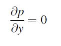
this means that pressure does not vary with respect to x. Similarly, for the y-direction we can assume the same as x-direction, hence:

These two equations show that there is no pressure variation in any lateral direction.

If we create a free body diagram for the z-direction and add up the forces, we obtain:

This shows that pressure does vary in a static fluid in the z-direction i.e., pressure increases with depth. This is mathematical shown by integrating both sides of the above equation:

where point 1 is a reference point such as the free surface of a liquid and point 2 is a point of interest. Since the density is a constant for incompressible fluids, we get: 

p₂ – p₁ = ρg(z₂ – z₁) = ρgΔz

where Δz is the depth below the liquid surface. This relationship is the basic equation of hydrostatics and is often written as:

Δp = ρgz