Fundamentals of Partial Differentiation of the Exact Differential Equation

Carrying out partial differentiation of the Exact Differential Equation of M and N with respect to z and y, respectively, results in:

dx is a perfect differential when the above equation is satisfied for any function x.

Similarly, if y = y(x, z) and z = z(x, y), then from these two relations, we have:

In terms of p, v and T, the following relation holds true:

Thermodynamic Relations

Some properties like temperature, pressure, volume, and mass can be measured directly while other properties like density and specific volume can be determined from these using some simple relations.

However, properties like internal energy, enthalpy, and entropy are not so easy to determine as they cannot be measured directly or related to easily measurable properties through some simple relations.

Thus, it is important to develop some fundamental relations between commonly encountered thermodynamic properties and express the properties that cannot be measured directly in terms of easily measurable properties.

Partial Derivatives and Associated Relations

Most basic thermodynamic relations involve differentials. Let us consider a function f that depends on a single variable x, i.e., f = f(x) as shown below:

The derivative of the function at a point defined as Slope expressed as:

Therefore, the derivative of a function f(x) with respect to x represents the rate of change of f with x.

Let us now consider a function that depends on two (or more) variables, such as z = z(x, y). This time the value of z depends on both x and y.

It is sometimes necessary to examine the dependence of z on only one of the variables by allowing one variable to change while holding the others constant and observing the change in the function.

The variation of z(x, y) with x when y is held constant is called the partial derivative of z with respect to x, and it is expressed as:

To obtain a relation for the total differential change in z(x, y) for simultaneous changes in x and y would be:

The above equation is the fundamental relation for the total differential of a dependent variable in terms of its partial derivatives with respect to the independent variables. This relation can easily be extended to include more independent variables.

An important relation for partial derivatives is used in calculus to test whether a differential dz is exact or inexact. In thermodynamics, this relation forms the basis for the development of the Maxwell relations which was discussed in a previous blog entry here where dz is replaced by dφ.

We can now develop two important relations for partial derivatives – the reciprocity and the cyclic relations.

The function z = z(x, y) can also be expressed as x = x(y, z) if y and z are taken to be the independent variables. Then the total differential of x becomes:

Eliminating dx from the above equation by combining the dz and dx equations we get:

The variables y and z are independent of each other and thus can be varied independently. For example, y can be held constant (dy = 0), and z can be varied over a range of values (dz ≠ 0). Therefore, for this equation to be valid at all times, the terms in the brackets must equal zero, regardless of the values of y and z. 

Setting the terms in each bracket of the above equation equal to zero gives two equations:

This equation is called the reciprocity relation, and it shows that the inverse of a partial derivative is equal to its reciprocal.

This equation is called the cyclic relation, and it is frequently used in thermodynamics.

SPECIAL MATHEMATICAL FUNCTIONS

Legendre’s Differential Equation

The differential equation, 

where n is a real constant known as Legendre’s equation of order n. When n is a nonnegative integer, i.e., n = 0, 1, 2, …., one solution of the above equation is called the Legendre polynomial (or Legendre function of the first kind) of degree n and is represented by P_n(x). The functions P_n(x) are expressed as follows:

Legendre polynomials are orthogonal with each other, i.e.,

The second solution of the Legendre equation is denoted by Q_n(x) and is called the Legendre function of the second kind of order n. The functions Q_n(x) are expressed as follows:

where A_n and B_n are suitably chosen constants. In particular:

Therefore, the general solution of Legendre’s differential equation is expressed as follows:

The substitution x = cos θ transforms Legendre’s equation into the following form:

The solution of Eq. (11) is given by

Legendre’s Associated Differential Equation

The differential equation:

where m and n are nonnegative integers, is known as Legendre’s associated equation of order n. Solutions of this equation are called associated Legendre functions. The general solution is:

where P_n^m (x) and Q_n^m (x) are called the associated Legendre function of the first kind and associated Legendre function of the second kind, respectively. Associated Legendre functions of the first kind are defined by:

Associated Legendre functions of the first kind are orthogonal with each other, i.e.,

Associated Legendre functions of the second kind are defined by:

The substitution x = cos θ transforms Legendre’s associated differential equation into the equation:

which is satisfied by P_n^m (cos θ) and Q_n^m (cos θ)

Hermite's Differential Equation

The differential equation:

where n is a real constant, is known as Hermite’s equation of order n. If n is a nonnegative integer, i.e., n = 0, 1, 2, ….. then solutions of Hermite’s equation are Hermite polynomials H_n(x) given by:

Hermite polynomials are orthogonal with each other, i.e.,

Laguerre's Differential Equation

The differential equation:

where n is a real constant, is known as Laguerre’s equation of order n. If n is a nonnegative integer, i.e., n = 0, 1, 2, ….., then solutions of Laguerre’s equation are Laguerre polynomials L_n(x) given by:

Laguerre polynomials are orthogonal with each other, i.e.,

Chebyshev's Differential Equation

The differential equation:

is known as Chebyshev’s equation of order n. The general solution of Chebyshev’s differential equation is:

where T_n(x) and S_n(x) are called the Chebyshev polynomials of the first kind and Chebyshev polynomials of the second kind, respectively. Chebyshev polynomial of the first kind is defined by:

Chebyshev polynomials of the first kind are orthogonal with each other, i.e.,

Chebyshev polynomial of the second kind S_n(x) is defined by:

Chebyshev polynomials of the second kind are orthogonal with each other, i.e.,

The Gaussian Integral

The Gaussian or Probability Integral is an essential concept in mathematics particularly in the fields of probability theory, statistics and quantum mechanics.

The Gaussian integral, closely related to the erf function, is the integral of the one-dimensional Gaussian function over (-∞, ∞).

The Gaussian Integral can also be defined as the integral of the exponential of -x² over the entire real line.

It can be calculated using the trick of combining two one-dimensional Gaussians:

In this case, Since the variable in the integral is a dummy variable i.e, it integrates out in the end, we can rename from x to y.

When switching to polar coordinates we get:

Example

Prove the following:

Solution

Convert the integral into the polar coordinates (r, θ) where x² + y² = r², 

and dxdy = rdrdθ:

Evaluating the integrals:

Therefore:

Laplace Transformation

Laplace transformations are a mathematical technique used to solve differential equations. Numerous mathematical problems are solved using transformations. The idea is to transform a difficult problem into another form that is easier to solve. Once the problem is solved, the inverse transform can be used to solve the original problem. 

The Laplace Transformation of a function f(t) can be converted into a function f(s) using the following equation:

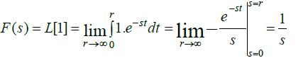
Example 1: Find the Laplace Transform of f(t) = 1

Solution:

Example 2: Find the Laplace Transform of f(t) = e^at

Solution:

Example 3: Find the Laplace Transform of f(t) = sin (wt) and f(t) = cos (wt) 

Solution:

Example 4: Find the Laplace Transform of f(t) = cosh (wt) and f(t) = sinh (wt)

Solution: 

Below is a summary table for common Laplace Transformations

Shifting Theorem

The common expression is as follows:

Example 5: Find the Laplace Transform of f(t) = e^at cos (bt)

Solution:

Example 6: Find the Laplace Transform of f(t) = sin (3t).e^5t 

Laplace Transforms for Derivatives

The following are the general equations for different ordered differential equations:

Example: Find the Laplace Transform of the function x(t) which satisfy the following differential equation and initial condition:

Solution:

Take the Laplace transform of both sides of the equation.

Laplace Transforms for Integrals 

The general equation for Laplace transforms of integrals is as follows:

Example: Find x(s) for the following equations

Solution