Entropy

Let us consider a closed system that undergoes a reversible process from an initial state, i, to a final state, f, using a process path. It is possible to draw an adiabatic and isothermal path from the initial and final state as shown:

The work done by the system going from the state i to f is the area under the process path on a P − V diagram. Between two adiabatic lines, it is possible to find an isothermal path gh such that the area under the curve ighf is equal to the actual work. This can be calculated as follows:

The above statements lead us to the theorem of Clausius which states:

Given any reversible process where the temperature changes in any prescribed manner, it is possible to find a reversible zigzag process that consists of adiabatic-isothermal-adiabatic steps such that the heat interaction in the isothermal step equals the heat interaction in the original process. 

Let us consider a system that undergoes a reversible and cyclic process with any two points, i and f, on a process path. The adiabatic lines that pass through these points intersect the cycle path at points c and d. Using the theorem of Clausius, it is possible to represent the paths i - f and d - c by adiabatic-isothermal-adiabatic paths as i - g - h - f and d - b - a - c, respectively in the following graph. Also note that Q_if = Q_gh and Q_dc = Q_ba

If we take the heat interaction of the path i – f, to be from a reservoir at T_H and in path d – c from a reservoir at T_C, we see that the cycle i-g-h-d-b-a-i is nothing but a Carnot cycle. Thus, using equation 21 from this blog entry, we can write:

An infinite number of infinitesimal cycles, beginning at j and ending at k, cover the entire cycle, we then obtain:

 

To evaluate ΔS for an irreversible process, we can devise a reversible path(s) between the same initial and final states and then evaluate dQ_rev/T over this reversible path

For an adiabatic and reversible process dQ_rev = 0 thus equation 11 simplifies as:

ΔS = 0                                     (12)

A process where the entropy remains constant is called an isentropic process. 

Statements of the Second Law of Thermodynamics

Clausius and Kelvin-Plank statements are the commonly accepted statements of the second law of thermodynamics. These statements are equivalent, and one necessarily implies the other.

Clausius Statement

It is impossible to construct a device operating in a cycle that produces no effect other than the transfer of heat from a cooler to a hotter body. Simply put, spontaneous heat transfer from a cooler body to a hotter body is not possible without any external work.

This is illustrated as follows:  

Kelvin-Plank statement

It is impossible to construct a device operating in a cycle that produces no effect other than the extraction of heat from a reservoir and the producing an equal amount of work. This is illustrated as follows: 

Example

Among the processes shown in below, identify the ones that are possible:

Solution

• Case 1: Heat flows spontaneously from hot to cold reservoir. From our everyday experience we know that this is possible.
• Case 2: Heat flows spontaneously from cold to hot reservoir. According to the Clausius statement this is impossible.
• Case 3: Work is completely converted to heat. This is possible.
• Case 4: Heat is completely converted into work. This phenomenon violates the Kelvin-Planck statement and hence, it is impossible.
• Case 5: Part of the heat received from a high-temperature reservoir is converted into work while the rest is discarded to a low-temperature reservoir. This represents a typical heat engine and it is possible.
• Case 6: Reverse of Case 5, i.e., work is done on the system, heat is transferred from a low-temperature reservoir to a high-temperature reservoir. Heat pumps (or, refrigerators) operate on this principle hence is possible.

Heat Engines and Heat Pumps

As previously defined, a heat engine is any mechanism operating cyclically with the primary aim of partially converting heat into work. The most efficient cycle is the Carnot heat engine which can operate between two constant heat reservoirs. The Carnot efficiency represents the upper limit.

A typical heat engine (shown below) produces high pressure steam in the boiler, expands it in the turbine to obtain work. The low-pressure steam exiting the turbine is sent to a condenser where heat is dissipated to the surroundings. Before the resultant liquid is returned to the boiler, its pressure is increased using a pump. A small amount of work obtained from the turbine is used in the pump.

The boiler-turbine-condenser-pump assembly can be represented as a circle in a schematic representation of a heat engine as shown below

A heat engine's performance is measured in terms of its efficiency, η, which is defined as:

Heat pumps are considered reversed heat engines, thus., they are used to transfer heat from a low temperature reservoir to a high temperature reservoir with the help of an external work. This can be schematically represented as follows: 

For a heat pump, its performance is measured using its coefficient of performance (COP) which is as follows:

Laplace Transformation

Laplace transformations are a mathematical technique used to solve differential equations. Numerous mathematical problems are solved using transformations. The idea is to transform a difficult problem into another form that is easier to solve. Once the problem is solved, the inverse transform can be used to solve the original problem. 

The Laplace Transformation of a function f(t) can be converted into a function f(s) using the following equation:

Example 1: Find the Laplace Transform of f(t) = 1

Solution:

Example 2: Find the Laplace Transform of f(t) = e^at

Solution:

Example 3: Find the Laplace Transform of f(t) = sin (wt) and f(t) = cos (wt) 

Solution:

Example 4: Find the Laplace Transform of f(t) = cosh (wt) and f(t) = sinh (wt)

Solution: 

Below is a summary table for common Laplace Transformations

Shifting Theorem

The common expression is as follows:

Example 5: Find the Laplace Transform of f(t) = e^at cos (bt)

Solution:

Example 6: Find the Laplace Transform of f(t) = sin (3t).e^5t 

Laplace Transforms for Derivatives

The following are the general equations for different ordered differential equations:

Example: Find the Laplace Transform of the function x(t) which satisfy the following differential equation and initial condition:

Solution:

Take the Laplace transform of both sides of the equation.

Laplace Transforms for Integrals 

The general equation for Laplace transforms of integrals is as follows:

Example: Find x(s) for the following equations

Solution

Introduction to Process Control

Process control can be defined the maintenance of a process output e.g., concentration, temperature or flow rate, within the desired specifications by continually adjusting other variables in that process. 

Some examples of controlled processes include:

• Controlling the temperature of a stream of water by controlling the amount of steam added into the shell of a heat exchanger.
• Isothermally operating a jacketed reactor by controlling the mixture of cold water and steam that flows through the jacket of the reactor.
• Maintenance of a set ratio of reactants to be added to a reactor by controlling their flow rates.
• Controlling the height of fluid in a tank to make sure it does not overflow.

Control System Objectives

• Safety
• Economic Incentives
• Increasing efficiency
• Ensuring process stability
• Elimination of routine
• Protection of equipment
• Reduction of variability
  

Important definitions in Process Control

System: This is a combination of components that collectively act and perform a certain objective.

Plant: This is the machine of which a particular quantity or condition is to be controlled.

Process: This is the changing or refining of raw materials that pass through or remain in a liquid, gaseous, or slurry state to create end products.

Control: in process industries, this refers to the regulation of all aspects of the process. Precise control of temperature, pressure, pH, level, oxygen, foam, nutrient, and flow is important in numerous process applications.

Sensor: This is a measuring instrument that detect the vale of the measurable variable as a function of time. The most common measurements are of flow (F), temperature (T), pressure (P), level (L), pH and composition (A, for analyzer).

Set point: This is the value at which the controlled parameter is to be maintained.

Controller: This is a device that receives a measurement of the process variable, compares it with a set point representing the desired control point, and adjusts its output to minimize the error between the measurement and the set point.

Error Signal: The signal resulting from the difference between the set point reference signal and the process variable feedback signal in a controller.

Feedback Control: A type of control where the controller receives a feedback signal representing the condition of the controlled process variable, then compares it to the set point and adjusts the controller output accordingly.

Steady-State: This is the condition when all of the process properties are constant with time, transient responses having died out.

Transmitter: This is a device that converts a process measurement (pressure, flow, level, temperature, etc.) into an electrical or pneumatic signal that is suitable for use by an indicating or control system.

Controlled variable: This is the process output that is to be maintained at a desired value by adjustment of a process input.

Manipulated variable: This is the process input that is to be adjusted to maintain the controlled output at set point.

Disturbance: This is a process input (other than the manipulated parameter) which affects the controlled parameter.

Process Time Constant (τ): This is an amount of time counted from the moment the variable starts to respond that it takes the process variable to reach 63.2% of its total change.

Block diagram: This is the relationship between the input and the output of the system. This is commonly illustrated as a figure. Examples are shown in the diagram below:

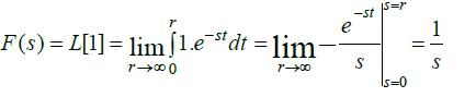
Transfer Function: This is the ratio of the Laplace transform of the output (response function) to the Laplace transform of the input (driving force) under the assumption that all the initial conditions are zero unless given another value.

Closed-loop control system: is a mechanical or electronic device that automatically regulates a system to maintain a desired state or set point without any human interaction. It uses a feedback system or sensor.

Advantage: more accurate than the open-loop control system.

Disadvantages: 

(1) Complex and expensive

(2) The stability is the major problem in closed-loop control system 

Open-loop control system: In this system there is no feedback to the controller about the current state of the system. There is no self-regulating mechanism and human interaction is typically required.

Advantages:

(1) Simple construction and ease of maintenance.

(2) Less expensive than closed-loop control system.

(3) There is no stability problem.

Disadvantages:

(1) Disturbance and change in calibration cause errors; and output may be different from what is  desired.

(2) To maintain the required quality in the output, recalibration is necessary from time to time

Carnot Cycle solved examples

For the following examples, equation from the previous blog entry are used. You can read them here.

Example 1

A Carnot cycle receives 1000 kJ of heat at 800°C and rejects heat at 300°C. Calculate the work output.

Solution

From Equation 23 of the Carnot Cycle blog entry:

      

Substituting the provided values into the above equation:

Thus:

W_net = 466 kJ

Example 2

Suppose an iceberg weighing 10¹⁰ kg drifts into the Gulf stream which has a temperature of 22°C. If we operate a Carnot heat engine using the Gulf stream as a heat source and the iceberg as a cold sink, what is the work output that could be generated while the iceberg is melting?

Solution

Assume that the temperature of the iceberg is 0°C and the heat of fusion for ice is 334,880 J/kg. Take the iceberg as the heat sink.

The amount of heat rejected to the sink is:

Q_C = (10¹⁰) (334,880) = 3.35 × 10¹⁵ J

The amount of heat absorbed can be calculated using equation 24: